Example notebooks
Begin exploring Enrich2 datasets with the following notebooks. They rely on the Enrich2 example dataset, so please perform that analysis before running any of these notebooks locally.
The notebooks can be run interactively by using the command line to navigate to the “Enrich2/docs/notebooks” directory and enter jupyter notebook <notebook.ipynb> where <notebook.ipynb> is the notebook file name.
The first two notebooks demonstrate using pandas to open an HDF5 file, extract its contents into a data frame, and perform queries on tables in the HDF5 file. For more information, see the pandas HDF5 documentation.
Selecting variants by input library count
This notebook gets scores and standard errors for the variants in a Selection that exceed a minimum count cutoff in the input time point, and plots the relationship between each variant’s score and input count.
% matplotlib inline
from __future__ import print_function
import os.path
import numpy as np
import pandas as pd
import matplotlib.pyplot as plt
from enrich2.variant import WILD_TYPE_VARIANT
import enrich2.plots as enrich_plot
pd.set_option("display.max_rows", 10) # rows shown when pretty-printing
Modify the results_path variable in the next cell to match the
output directory of your Enrich2-Example dataset.
results_path = "/path/to/Enrich2-Example/Results/"
Open the Selection HDF5 file with the variants we are interested in.
my_store = pd.HDFStore(os.path.join(results_path, "Rep1_sel.h5"))
The pd.HDFStore.keys() method returns a list of all the tables in
this HDF5 file.
my_store.keys()
['/main/barcodemap',
 '/main/barcodes/counts',
 '/main/barcodes/counts_unfiltered',
 '/main/barcodes/log_ratios',
 '/main/barcodes/scores',
 '/main/barcodes/weights',
 '/main/synonymous/counts',
 '/main/synonymous/counts_unfiltered',
 '/main/synonymous/log_ratios',
 '/main/synonymous/scores',
 '/main/synonymous/weights',
 '/main/variants/counts',
 '/main/variants/counts_unfiltered',
 '/main/variants/log_ratios',
 '/main/variants/scores',
 '/main/variants/weights']
We will work with the “/main/variants/counts” table first. Enrich2
names the columns for counts c_n where n is the time point,
beginning with 0 for the input library.
We can use a query to extract the subset of variants in the table that
exceed the specified cutoff. Since we’re only interested in variants,
we’ll explicitly exclude the wild type. We will store the data we
extract in the variant_count data frame.
read_cutoff = 10
variant_counts = my_store.select('/main/variants/counts', where='c_0 > read_cutoff and index != WILD_TYPE_VARIANT')
variant_counts
| c_0 | c_2 | c_5 | |
|---|---|---|---|
| c.10G>A (p.Ala4Arg), c.11C>G (p.Ala4Arg), c.12T>A (p.Ala4Arg) | 787.0 | 106.0 | 124.0 |
| c.10G>A (p.Ala4Asn), c.11C>A (p.Ala4Asn) | 699.0 | 80.0 | 114.0 |
| c.10G>A (p.Ala4Asn), c.11C>A (p.Ala4Asn), c.12T>C (p.Ala4Asn) | 94.0 | 8.0 | 13.0 |
| c.10G>A (p.Ala4Ile), c.11C>T (p.Ala4Ile) | 1280.0 | 137.0 | 80.0 |
| c.10G>A (p.Ala4Ile), c.11C>T (p.Ala4Ile), c.12T>A (p.Ala4Ile) | 717.0 | 42.0 | 27.0 |
| ... | ... | ... | ... |
| c.9T>A (p.=) | 327.0 | 217.0 | 284.0 |
| c.9T>C (p.=) | 1947.0 | 523.0 | 1230.0 |
| c.9T>C (p.=), c.49A>T (p.Met17Ser), c.50T>C (p.Met17Ser), c.51G>A (p.Met17Ser) | 277.0 | 43.0 | 5.0 |
| c.9T>C (p.=), c.62T>C (p.Leu21Ser), c.63A>T (p.Leu21Ser) | 495.0 | 138.0 | 55.0 |
| c.9T>G (p.=) | 406.0 | 18.0 | 20.0 |
1440 rows × 3 columns
The index of the data frame is the list of variants that exceeded the cutoff.
variant_counts.index
Index([u'c.10G>A (p.Ala4Arg), c.11C>G (p.Ala4Arg), c.12T>A (p.Ala4Arg)',
       u'c.10G>A (p.Ala4Asn), c.11C>A (p.Ala4Asn)',
       u'c.10G>A (p.Ala4Asn), c.11C>A (p.Ala4Asn), c.12T>C (p.Ala4Asn)',
       u'c.10G>A (p.Ala4Ile), c.11C>T (p.Ala4Ile)',
       u'c.10G>A (p.Ala4Ile), c.11C>T (p.Ala4Ile), c.12T>A (p.Ala4Ile)',
       u'c.10G>A (p.Ala4Ile), c.11C>T (p.Ala4Ile), c.12T>C (p.Ala4Ile)',
       u'c.10G>A (p.Ala4Lys), c.11C>A (p.Ala4Lys), c.12T>A (p.Ala4Lys)',
       u'c.10G>A (p.Ala4Met), c.11C>T (p.Ala4Met), c.12T>G (p.Ala4Met)',
       u'c.10G>A (p.Ala4Ser), c.11C>G (p.Ala4Ser)',
       u'c.10G>A (p.Ala4Ser), c.11C>G (p.Ala4Ser), c.12T>C (p.Ala4Ser)',
       ...
       u'c.8C>T (p.Ser3Phe), c.60C>T (p.=)',
       u'c.8C>T (p.Ser3Phe), c.9T>C (p.Ser3Phe)', u'c.90C>A (p.=)',
       u'c.90C>G (p.Ile30Met)', u'c.90C>T (p.=)', u'c.9T>A (p.=)',
       u'c.9T>C (p.=)',
       u'c.9T>C (p.=), c.49A>T (p.Met17Ser), c.50T>C (p.Met17Ser), c.51G>A (p.Met17Ser)',
       u'c.9T>C (p.=), c.62T>C (p.Leu21Ser), c.63A>T (p.Leu21Ser)',
       u'c.9T>G (p.=)'],
      dtype='object', length=1440)
We can use this index to get the scores for these variants by querying
the “/main/variants/scores” table. We’ll store the result of the query
in a new data frame named variant_scores, and keep only the score
and standard error (SE) columns.
variant_scores = my_store.select('/main/variants/scores', where='index in variant_counts.index')
variant_scores = variant_scores[['score', 'SE']]
variant_scores
| score | SE | |
|---|---|---|
| c.10G>A (p.Ala4Arg), c.11C>G (p.Ala4Arg), c.12T>A (p.Ala4Arg) | -0.980091 | 0.134873 |
| c.10G>A (p.Ala4Asn), c.11C>A (p.Ala4Asn) | -0.972035 | 0.268962 |
| c.10G>A (p.Ala4Asn), c.11C>A (p.Ala4Asn), c.12T>C (p.Ala4Asn) | -1.138667 | 0.403767 |
| c.10G>A (p.Ala4Ile), c.11C>T (p.Ala4Ile) | -1.875331 | 0.014883 |
| c.10G>A (p.Ala4Ile), c.11C>T (p.Ala4Ile), c.12T>A (p.Ala4Ile) | -2.552289 | 0.421699 |
| ... | ... | ... |
| c.9T>A (p.=) | 0.705661 | 0.774559 |
| c.9T>C (p.=) | 0.438654 | 0.014857 |
| c.9T>C (p.=), c.49A>T (p.Met17Ser), c.50T>C (p.Met17Ser), c.51G>A (p.Met17Ser) | -1.930922 | 1.085535 |
| c.9T>C (p.=), c.62T>C (p.Leu21Ser), c.63A>T (p.Leu21Ser) | -0.897249 | 0.884321 |
| c.9T>G (p.=) | -2.314604 | 0.671760 |
1440 rows × 2 columns
Now that we’re finished getting data out of the HDF5 file, we’ll close it.
my_store.close()
To more easily explore the relationship between input count and score,
we’ll add a column to the variant_scores data frame that contains
input counts from the variant_counts data frame.
variant_scores['input_count'] = variant_counts['c_0']
variant_scores
| score | SE | input_count | |
|---|---|---|---|
| c.10G>A (p.Ala4Arg), c.11C>G (p.Ala4Arg), c.12T>A (p.Ala4Arg) | -0.980091 | 0.134873 | 787.0 |
| c.10G>A (p.Ala4Asn), c.11C>A (p.Ala4Asn) | -0.972035 | 0.268962 | 699.0 |
| c.10G>A (p.Ala4Asn), c.11C>A (p.Ala4Asn), c.12T>C (p.Ala4Asn) | -1.138667 | 0.403767 | 94.0 |
| c.10G>A (p.Ala4Ile), c.11C>T (p.Ala4Ile) | -1.875331 | 0.014883 | 1280.0 |
| c.10G>A (p.Ala4Ile), c.11C>T (p.Ala4Ile), c.12T>A (p.Ala4Ile) | -2.552289 | 0.421699 | 717.0 |
| ... | ... | ... | ... |
| c.9T>A (p.=) | 0.705661 | 0.774559 | 327.0 |
| c.9T>C (p.=) | 0.438654 | 0.014857 | 1947.0 |
| c.9T>C (p.=), c.49A>T (p.Met17Ser), c.50T>C (p.Met17Ser), c.51G>A (p.Met17Ser) | -1.930922 | 1.085535 | 277.0 |
| c.9T>C (p.=), c.62T>C (p.Leu21Ser), c.63A>T (p.Leu21Ser) | -0.897249 | 0.884321 | 495.0 |
| c.9T>G (p.=) | -2.314604 | 0.671760 | 406.0 |
1440 rows × 3 columns
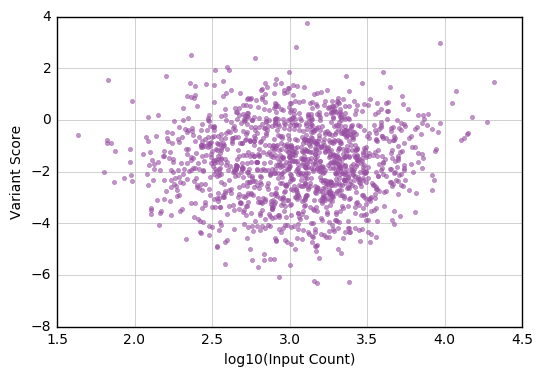
Now that all the information is in a single data frame, we can make a plot of score vs. input count. This example uses functions and colors from the Enrich2 plotting library. Taking the log10 of the counts makes the data easier to visualize.
fig, ax = plt.subplots()
enrich_plot.configure_axes(ax, xgrid=True)
ax.plot(np.log10(variant_scores['input_count']),
        variant_scores['score'],
        linestyle='none', marker='.', alpha=0.6,
        color=enrich_plot.plot_colors['bright4'])
ax.set_xlabel("log10(Input Count)")
ax.set_ylabel("Variant Score")
<matplotlib.text.Text at 0x9e796a0>
Selecting variants by number of unique barcodes
This notebook gets scores for the variants in an Experiment that are linked to multiple barcodes, and plots the relationship between each variant’s score and number of unique barcodes.
% matplotlib inline
from __future__ import print_function
import os.path
from collections import Counter
import numpy as np
import pandas as pd
import matplotlib.pyplot as plt
from enrich2.variant import WILD_TYPE_VARIANT
import enrich2.plots as enrich_plot
pd.set_option("display.max_rows", 10) # rows shown when pretty-printing
Modify the results_path variable in the next cell to match the
output directory of your Enrich2-Example dataset.
results_path = "/path/to/Enrich2-Example/Results/"
Open the Experiment HDF5 file.
my_store = pd.HDFStore(os.path.join(results_path, "BRCA1_Example_exp.h5"))
The pd.HDFStore.keys() method returns a list of all the tables in
this HDF5 file.
my_store.keys()
['/main/barcodemap',
 '/main/barcodes/counts',
 '/main/barcodes/scores',
 '/main/barcodes/scores_shared',
 '/main/barcodes/scores_shared_full',
 '/main/synonymous/counts',
 '/main/synonymous/scores',
 '/main/synonymous/scores_pvalues_wt',
 '/main/synonymous/scores_shared',
 '/main/synonymous/scores_shared_full',
 '/main/variants/counts',
 '/main/variants/scores',
 '/main/variants/scores_pvalues_wt',
 '/main/variants/scores_shared',
 '/main/variants/scores_shared_full']
First we will work with the barcode-variant map for this analysis, stored in the “/main/barcodemap” table. The index is the barcode and it has a single column for the variant HGVS string.
bcm = my_store['/main/barcodemap']
bcm
| value | |
|---|---|
| TTTTTTGTGTCTGTGA | _wt |
| GGGCACGTCTTTATAG | _wt |
| GTTACTGGTTAGTATT | _wt |
| GTTACTTGATCCGACC | _wt |
| GTTAGATGGATGTACG | _wt |
| ... | ... |
| GAGTACTTTTTTGATT | c.9T>C (p.=), c.62T>C (p.Leu21Ser), c.63A>T (p... |
| ATGATGACGTGTCTTG | c.9T>G (p.=) |
| TCACCGGAACGTTGGT | c.9T>G (p.=) |
| TGACGATGTTGCATTT | c.9T>G (p.=), c.17G>C (p.Arg6Pro), c.18C>T (p.... |
| GTTATCAGCGCCCCTT | c.9T>G (p.=), c.85T>G (p.Leu29Gly), c.86T>G (p... |
20325 rows × 1 columns
To find out how many unique barcodes are linked to each variant, we’ll count the number of times each variant appears in the barcode-variant map using a Counter data structure. We’ll then output the top ten variants by number of unique barcodes.
variant_bcs = Counter(bcm['value'])
variant_bcs.most_common(10)
[('_wt', 5844),
 ('c.63A>T (p.Leu21Phe)', 109),
 ('c.39C>A (p.=)', 91),
 ('c.61T>A (p.Leu21Ile), c.63A>T (p.Leu21Ile)', 77),
 ('c.62T>A (p.Leu21Tyr), c.63A>T (p.Leu21Tyr)', 77),
 ('c.63A>G (p.=)', 73),
 ('c.72C>A (p.=)', 72),
 ('c.62T>G (p.Leu21Cys), c.63A>T (p.Leu21Cys)', 71),
 ('c.13C>A (p.Leu5Ile)', 70),
 ('c.62T>A (p.Leu21Ter)', 63)]
Next we’ll turn the Counter into a data frame.
bc_counts = pd.DataFrame(variant_bcs.most_common(), columns=['variant', 'barcodes'])
bc_counts
| variant | barcodes | |
|---|---|---|
| 0 | _wt | 5844 |
| 1 | c.63A>T (p.Leu21Phe) | 109 |
| 2 | c.39C>A (p.=) | 91 |
| 3 | c.61T>A (p.Leu21Ile), c.63A>T (p.Leu21Ile) | 77 |
| 4 | c.62T>A (p.Leu21Tyr), c.63A>T (p.Leu21Tyr) | 77 |
| ... | ... | ... |
| 1958 | c.77G>T (p.Cys26Leu), c.78C>A (p.Cys26Leu), c.... | 1 |
| 1959 | c.67T>A (p.Cys23Ile), c.68G>T (p.Cys23Ile), c.... | 1 |
| 1960 | c.41T>C (p.Ile14Thr), c.48T>G (p.=) | 1 |
| 1961 | c.55A>C (p.Lys19Leu), c.56A>T (p.Lys19Leu), c.... | 1 |
| 1962 | c.50T>C (p.Met17Thr), c.78C>T (p.=) | 1 |
1963 rows × 2 columns
The data frame has the information we want, but it will be easier to use later if it’s indexed by variant rather than row number.
bc_counts.index = bc_counts['variant']
bc_counts.index.name = None
del bc_counts['variant']
bc_counts
| barcodes | |
|---|---|
| _wt | 5844 |
| c.63A>T (p.Leu21Phe) | 109 |
| c.39C>A (p.=) | 91 |
| c.61T>A (p.Leu21Ile), c.63A>T (p.Leu21Ile) | 77 |
| c.62T>A (p.Leu21Tyr), c.63A>T (p.Leu21Tyr) | 77 |
| ... | ... |
| c.77G>T (p.Cys26Leu), c.78C>A (p.Cys26Leu), c.81G>T (p.=) | 1 |
| c.67T>A (p.Cys23Ile), c.68G>T (p.Cys23Ile), c.69T>A (p.Cys23Ile) | 1 |
| c.41T>C (p.Ile14Thr), c.48T>G (p.=) | 1 |
| c.55A>C (p.Lys19Leu), c.56A>T (p.Lys19Leu), c.57A>G (p.Lys19Leu), c.81G>T (p.=) | 1 |
| c.50T>C (p.Met17Thr), c.78C>T (p.=) | 1 |
1963 rows × 1 columns
We’ll use a cutoff to choose variants with a minimum number of unique barcodes, and store this subset in a new index. We’ll also exclude the wild type by dropping the first entry of the index.
bc_cutoff = 10
multi_bc_variants = bc_counts.loc[bc_counts['barcodes']  >= bc_cutoff].index[1:]
multi_bc_variants
Index([u'c.63A>T (p.Leu21Phe)', u'c.39C>A (p.=)',
       u'c.61T>A (p.Leu21Ile), c.63A>T (p.Leu21Ile)',
       u'c.62T>A (p.Leu21Tyr), c.63A>T (p.Leu21Tyr)', u'c.63A>G (p.=)',
       u'c.72C>A (p.=)', u'c.62T>G (p.Leu21Cys), c.63A>T (p.Leu21Cys)',
       u'c.13C>A (p.Leu5Ile)', u'c.62T>A (p.Leu21Ter)',
       u'c.63A>C (p.Leu21Phe)',
       ...
       u'c.88A>C (p.Ile30Arg), c.89T>G (p.Ile30Arg), c.90C>T (p.Ile30Arg)',
       u'c.76T>A (p.Cys26Lys), c.77G>A (p.Cys26Lys), c.78C>G (p.Cys26Lys)',
       u'c.22G>A (p.Glu8Ile), c.23A>T (p.Glu8Ile), c.24A>T (p.Glu8Ile)',
       u'c.49A>T (p.Met17Ser), c.50T>C (p.Met17Ser), c.51G>A (p.Met17Ser)',
       u'c.64G>A (p.Glu22Arg), c.65A>G (p.Glu22Arg)',
       u'c.77G>C (p.Cys26Ser), c.78C>G (p.Cys26Ser)',
       u'c.29T>A (p.Val10Glu), c.30A>G (p.Val10Glu)',
       u'c.50T>A (p.Met17Asn), c.51G>T (p.Met17Asn)',
       u'c.61T>A (p.Leu21Thr), c.62T>C (p.Leu21Thr), c.63A>G (p.Leu21Thr)',
       u'c.49A>G (p.Met17Ala), c.50T>C (p.Met17Ala)'],
      dtype='object', length=504)
We can use this index to get condition-level scores for these variants by querying the “/main/variants/scores” table. Since we are working with an Experiment HDF5 file, the data frame column names are a MultiIndex with two levels, one for experimental conditions and one for data values (see the pandas documentation for more information).
multi_bc_scores = my_store.select('/main/variants/scores', where='index in multi_bc_variants')
multi_bc_scores
| condition | E3 | ||
|---|---|---|---|
| value | SE | epsilon | score |
| c.10G>A (p.Ala4Thr) | 1.435686e-01 | 3.469447e-18 | -0.238174 |
| c.10G>T (p.Ala4Ser) | 1.456404e-29 | 2.087042e-57 | -0.177983 |
| c.11C>A (p.Ala4Asp) | 5.309592e-01 | 1.110223e-16 | 0.027898 |
| c.13C>A (p.Leu5Ile) | 1.333666e-01 | 0.000000e+00 | -0.623652 |
| c.13C>A (p.Leu5Ser), c.14T>G (p.Leu5Ser) | 3.612046e-01 | 2.775558e-17 | 0.657916 |
| ... | ... | ... | ... |
| c.89T>G (p.Ile30Ser), c.90C>T (p.Ile30Ser) | 6.069463e-01 | 0.000000e+00 | -0.826140 |
| c.8C>A (p.Ser3Tyr) | 3.785724e-01 | 2.775558e-17 | -1.440477 |
| c.8C>T (p.Ser3Phe) | 8.669053e-02 | 2.602085e-18 | -0.091250 |
| c.90C>A (p.=) | 9.681631e-02 | 5.204170e-18 | -0.217977 |
| c.90C>T (p.=) | 5.450037e-117 | 8.793373e-229 | 0.805631 |
486 rows × 3 columns
There are fewer rows in multi_bc_scores than in
multi_bc_variants because some of the variants were not scored in
all replicate selections, and therefore do not have a condition-level
score.
Now that we’re finished getting data out of the HDF5 file, we’ll close it.
my_store.close()
We’ll add a column to the bc_counts data frame that contains scores
from the multi_bc_scores data frame. To reference a column in a data
frame with a MultiIndex, we need to specify all column levels.
bc_counts['score'] = multi_bc_scores['E3', 'score']
bc_counts
| barcodes | score | |
|---|---|---|
| _wt | 5844 | NaN |
| c.63A>T (p.Leu21Phe) | 109 | 1.387659 |
| c.39C>A (p.=) | 91 | -0.189253 |
| c.61T>A (p.Leu21Ile), c.63A>T (p.Leu21Ile) | 77 | -1.031977 |
| c.62T>A (p.Leu21Tyr), c.63A>T (p.Leu21Tyr) | 77 | 0.310854 |
| ... | ... | ... |
| c.77G>T (p.Cys26Leu), c.78C>A (p.Cys26Leu), c.81G>T (p.=) | 1 | NaN |
| c.67T>A (p.Cys23Ile), c.68G>T (p.Cys23Ile), c.69T>A (p.Cys23Ile) | 1 | NaN |
| c.41T>C (p.Ile14Thr), c.48T>G (p.=) | 1 | NaN |
| c.55A>C (p.Lys19Leu), c.56A>T (p.Lys19Leu), c.57A>G (p.Lys19Leu), c.81G>T (p.=) | 1 | NaN |
| c.50T>C (p.Met17Thr), c.78C>T (p.=) | 1 | NaN |
1963 rows × 2 columns
Many rows in bc_counts are missing scores (displayed as NaN) because
those variants were not in multi_bc_scores. We’ll drop them before
continuing.
bc_counts.dropna(inplace=True)
bc_counts
| barcodes | score | |
|---|---|---|
| c.63A>T (p.Leu21Phe) | 109 | 1.387659 |
| c.39C>A (p.=) | 91 | -0.189253 |
| c.61T>A (p.Leu21Ile), c.63A>T (p.Leu21Ile) | 77 | -1.031977 |
| c.62T>A (p.Leu21Tyr), c.63A>T (p.Leu21Tyr) | 77 | 0.310854 |
| c.63A>G (p.=) | 73 | -0.406277 |
| ... | ... | ... |
| c.64G>A (p.Glu22Arg), c.65A>G (p.Glu22Arg) | 10 | -2.577200 |
| c.77G>C (p.Cys26Ser), c.78C>G (p.Cys26Ser) | 10 | -3.497939 |
| c.50T>A (p.Met17Asn), c.51G>T (p.Met17Asn) | 10 | -1.737378 |
| c.61T>A (p.Leu21Thr), c.62T>C (p.Leu21Thr), c.63A>G (p.Leu21Thr) | 10 | -1.307432 |
| c.49A>G (p.Met17Ala), c.50T>C (p.Met17Ala) | 10 | -1.958962 |
486 rows × 2 columns
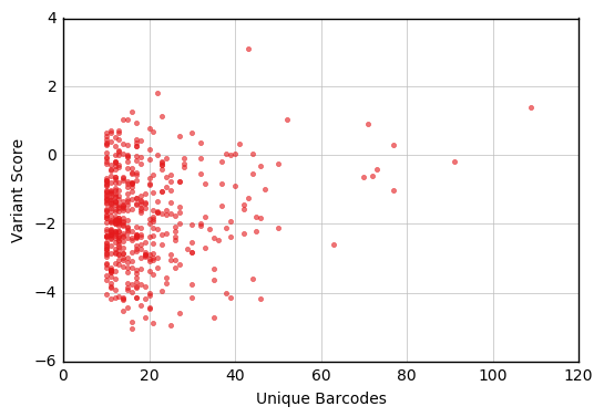
Now that we have a data frame containing the subset of variants we’re interested in, we can make a plot of score vs. number of unique barcodes. This example uses functions and colors from the Enrich2 plotting library.
fig, ax = plt.subplots()
enrich_plot.configure_axes(ax, xgrid=True)
ax.plot(bc_counts['barcodes'],
        bc_counts['score'],
        linestyle='none', marker='.', alpha=0.6,
        color=enrich_plot.plot_colors['bright5'])
ax.set_xlabel("Unique Barcodes")
ax.set_ylabel("Variant Score")
<matplotlib.text.Text at 0xd91fe80>
For more information on Enrich2 data tables, see Output HDF5 files.